Standard Curve Method for ELISA
Generally speaking, the standard fitting curve of ELISA is based on the classic software of Curve Expert 1.3 or Curve Expert 1.4. Now we will use the Curve Expert 1.4 to illustrate how to construct the ELISA standard curve.
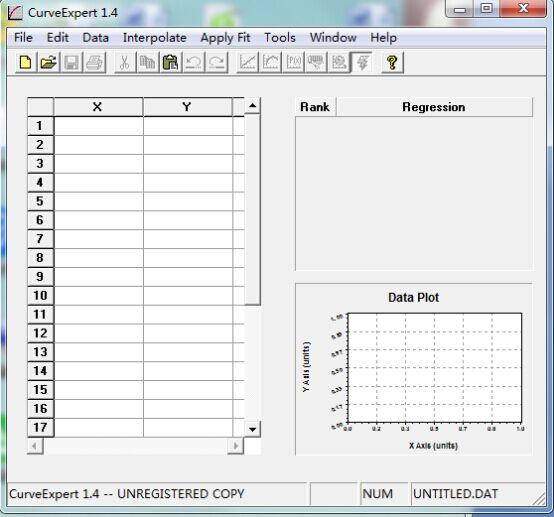
1.Click Curve Expert 1.4, and then open the application programs. You will see the following screen shot.
 &
&
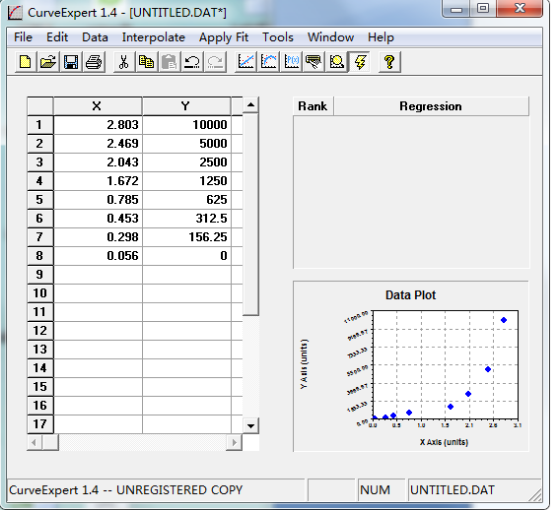
2. Input the value of OD on the X-axis against the concentration of samples on the Y-axis. The following screen shot will appear like this.
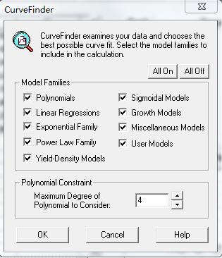
3. Click the icon showed on the above screen shot and you will see the following picture.
 &
&
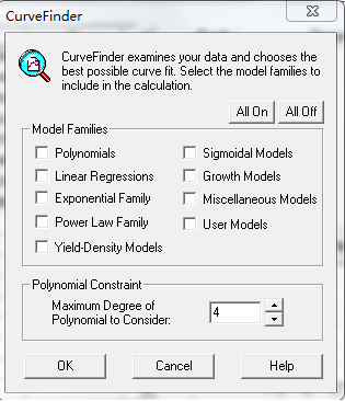
4. Click the ‘All Off’ button , you can see the following screen shot.
5. We select the Sigmoidal Models to fit the ELISA standard curve. Click ‘OK’ ,and you will see the following screen shot.
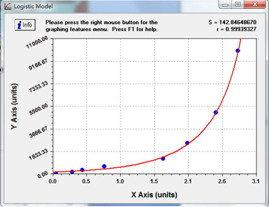
Please note that the higher the r-value in the above picture ( or the closer the r-value is to 1), the more reliable values you will get.
6. Please press the Ctrl plus L in the blank part of the above picture . The interface will appear like this.
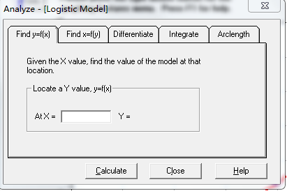

After inputting the corresponding OD-value (x-value), click the button “Calculate”.The concentration (Y-value)of samples can be measured. The final concentration can be obtained by multiplying the the measured figure with the times the samples have been diluted.
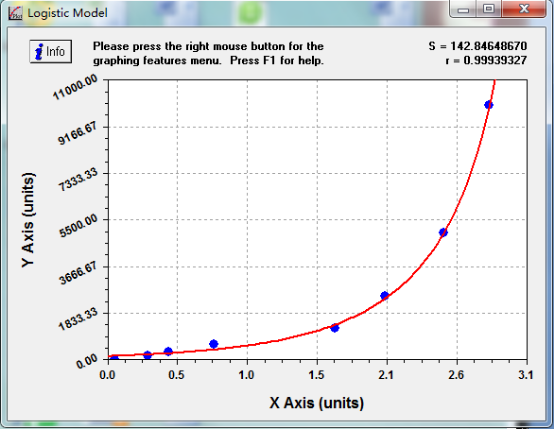
7. Click the button on the top left corner in the picture. Then you can get the ELISA curve fitting equation as follows.
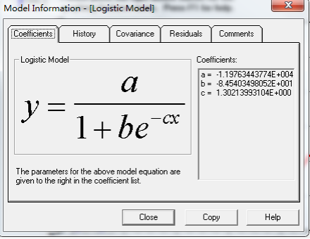
8. Logistic Model: y=a/(1+b*exp(-cx))
Coefficient Data:
a = -1.19763443774E+004
b = -8.45403498052E+001
c = 1.30213993104E+000
Click the button “copy” and you will get the figures for curve equation showed in the above screen shot.
Logistic Model: y=a/(1+b*exp(-cx))
Coefficient Data:
a = -1.19763443774E+004
b = -8.45403498052E+001
c = 1.30213993104E+000
1.Click Curve Expert 1.4, and then open the application programs. You will see the following screen shot.
 &
& 2. Input the value of OD on the X-axis against the concentration of samples on the Y-axis. The following screen shot will appear like this.

3. Click the icon
 showed on the above screen shot and you will see the following picture.
 &
& 4. Click the ‘All Off’ button , you can see the following screen shot.

5. We select the Sigmoidal Models to fit the ELISA standard curve. Click ‘OK’ ,and you will see the following screen shot.

Please note that the higher the r-value in the above picture ( or the closer the r-value is to 1), the more reliable values you will get.
6. Please press the Ctrl plus L in the blank part of the above picture . The interface will appear like this.


After inputting the corresponding OD-value (x-value), click the button “Calculate”.The concentration (Y-value)of samples can be measured. The final concentration can be obtained by multiplying the the measured figure with the times the samples have been diluted.
7. Click the button
 on the top left corner in the picture. Then you can get the ELISA curve fitting equation as follows.

8. Logistic Model: y=a/(1+b*exp(-cx))
Coefficient Data:
a = -1.19763443774E+004
b = -8.45403498052E+001
c = 1.30213993104E+000
Click the button “copy” and you will get the figures for curve equation showed in the above screen shot.
Logistic Model: y=a/(1+b*exp(-cx))
Coefficient Data:
a = -1.19763443774E+004
b = -8.45403498052E+001
c = 1.30213993104E+000


